A first look at DSOs
This introduction to digital storage oscilloscopes (DSOs) takes you on a quick but comprehensive tour of DSO functions and measurements.
Published with permission from Fluke An oscilloscope measures and displays voltage signals on a time-versus-voltage graph. In most applications the graph shows how the signal changes over time: the vertical (Y) axis represents voltage, and the horizontal (X) axis represents time. This simple graph can tell you many things about a signal:
• View the signal for glitches.
• Calculate the frequency of an oscillating signal.
• Tell if a malfunctioning component is distorting the signal.
• Tell how much of the signal is noise and whether the noise is changing with time.
Today’s handheld digital storage oscilloscopes offer two critical advantages over benchtop models: they are battery-operated, and they use isolated, electrically floating inputs. These designs make safety-certified measurements possible in 1000V CAT II and 600V CAT III environments — a critical need for safely troubleshooting electrical devices in high-energy applications.
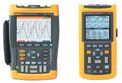 | Far left: The Fluke 190 Series ScopeMeter has a 200 MHz bandwidth and 2.5 GS/s real-time sampling rate. Left: The Fluke 123 ScopeMeter with 20 MHz dual-input measurement shows both meter reading and waveform. |
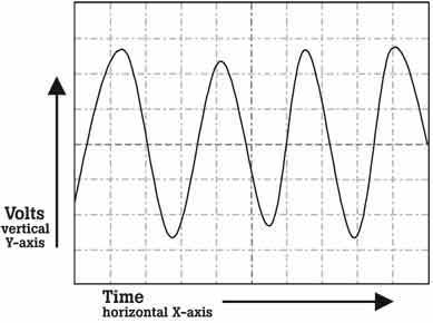 | Figure 1. Time-versus-voltage graph. |
Scopes and DMMs
The difference between an oscilloscope and a DMM (digital multimeter) can be summarily stated as “pictures vs. numbers.” A DMM is a tool for making precise measurements of discrete signals, enabling readings of up to eight digits of resolution for the voltage, current or frequency of a signal. On the other hand, it cannot depict waveforms visually to reveal signal strength, waveshape, or the instantaneous value of the signal. Nor is it equipped to reveal a transient or a harmonic signal that could compromise the operation of a system.
A scope adds a wealth of information to the numeric readings of a DMM. While displaying instantaneous numerical values of a wave, it also reveals the shape of the wave, including its amplitude (voltage) and frequency. With such visual information, a transient signal that may pose major consequences to a system can be displayed, measured and isolated.
Reach for a scope if you want to make both quantitative and qualitative measurements. Use a DMM to make high-precision checks of voltage, current, resistance and other electrical parameters.
Sampling
Sampling is the process of converting a portion of an input signal into a number of discrete electrical values for the purpose of storage, processing and display. The magnitude of each sampled point is equal to the amplitude of the input signal at the time the signal is sampled. The input waveform appears as a series of dots on the display. If the dots are widely spaced and difficult to interpret as a waveform, they can be connected using a process called interpolation, which connects the dots with lines, or vectors.
Triggering
Trigger controls allow you to stabilize and display a repetitive waveform.
Edge triggering is the most common form of triggering. In this mode, the trigger level and slope controls provide the basic trigger point definition. The slope control determines whether the trigger point is on the rising or the falling edge of a signal, and the level control determines where on the edge the trigger point occurs.
For even greater control and visibility into signal phenomena, you can use the ability of some DSOs to capture events leading up to the trigger point (“pre-trigger”) or after the trigger point (“posttrigger”) on the input waveform. As one example, by using pretriggering or post-triggering, you may catch a spike that occurs in between two occurrences of a signal.
Pulse width triggering triggers on specific pulses within a series or it can identify one-time or sporadic problems in a pulsed signal. In this mode, you can monitor a signal indefinitely and trigger on the first occurrence of a pulse whose duration, or pulse width, is either outside of or within set limits. The goal is to isolate and display a pulse that meets the predetermined time criteria.
Single-shot triggering is useful for capturing a one-time event — such as electrical arcing or a relay closure. A DSO with a single-shot mode waits until it receives a trigger and then sets itself in a hold mode to store the signal at the moment the onetime event occurs.
Video triggering is a powerful feature of advanced DSOs. Video signals can be extremely complex, providing no unique edge that is repetitive and that can be isolated to stabilize the signal. With an extensive range of signaling protocols in use in today’s electronicvideo equipment and systems, an effective DSO is one that recognizes the predominant video protocols and provides appropriate triggering functionality.
 | Figure 2. Sampling and interpolation. |
Setup The task of capturing and analyzing an unknown waveform on an oscilloscope can be routine, or it can seem like taking a shot in the dark. However, in most cases, taking a methodical approach to setting the oscilloscope will capture a stable waveform or help you determine how the scope controls need to be set so that you can capture the waveform.
1) Start with Auto Connect the ground reference lead and then connect the probe tip to the circuit test point. Most oscilloscopes have the ability to either perform a one-time auto setup or continuously analyze the unknown input signal. Press the AUTO button or verify that the scope is already in Auto mode.
Pressing the AUTO button will typically set up the oscilloscope to automatically adjust three key parameters:
Vertical sensitivity. Adjusts the vertical sensitivity so that the vertical amplitude spans approximately three to six divisions.
 | Figure 3. Unknown trace adjusted for 3-6 vertical divisions. |
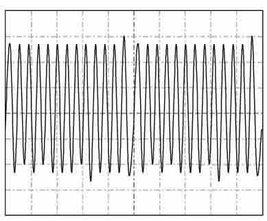
Horizontal timing. Adjusts the horizontal time per division so that there are three to four periods of the waveform across the width of the display.
 | Figure 4. Unknown trace adjusted for 3-4 periods horizontally. |
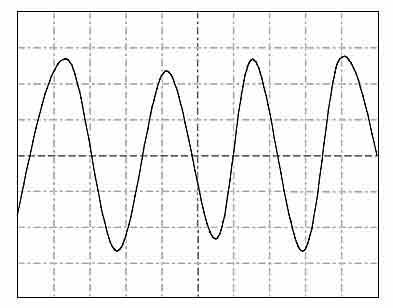
Trigger position. Sets the trigger position to the 50 % point of the vertical amplitude. Depending on the signal characteristics, this action may or may not result in a stable display.
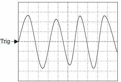 | Figure 5a. Trigger point set to 50% point on trace. |
 | Figure 5b. Trigger point is set to the 50 % point but due to the aberration on the leading edge in the second period, an additional trigger results in an unstable display. |
At this point you should see a trace that 1) lies within the vertical range of the display, 2) shows at least three periods of a waveform, and 3) is stable enough to allow you to recognize the overall characteristics of the waveform. Next, start fine-tuning the settings.
2) Adjust vertical and horizontal settings Start by adjusting the horizontal timing, increasing the time per division so that you see a wide time span of the unknown waveform. From that view, reverse the adjustment as required to narrow the view to just what you want to display.
Now adjust the vertical sensitivity, expanding the waveform vertically but ensuring that the high and low points of the waveform do not exceed the vertical span.
3) Adjust trigger settings If needed, adjust the trigger settings to stabilize the waveform display. Or, you may want to adjust the trigger delay to see pre- or post-trigger details on the waveform. Always start with the trigger-level setting, adjusting it so that it falls on a repetitive, unique point on the rising or falling edge of a waveform.
As an example, with the oscilloscope trigger set to the rising edge and the level set to the 50 % point, the following figures illustrate the cause of an unstable waveform display.
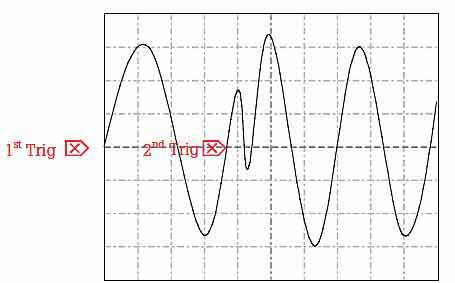 | Figure 6a. At the first update, the scope triggers on the first edge. On the second update, the scope may trigger on the second trigger point indicated. |
After two successive updates based on triggers 1 and 2, the resultant trace will appear unstable.
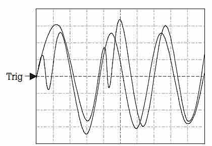 | Figure 6b. Unstable waveform display caused by incorrect trigger level setting. |
However, simply by manually adjusting the trigger point to a repetitive, unique point on the edge, you can solve this problem and produce a stable waveform display.
 | Figure 6c. Trigger level adjusted to a unique repetitive position, outside the aberration on the second period. |
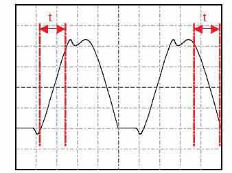
When working with complex signals like a series of pulses, pulse width triggering may be required. With this technique, both the trigger-level setting and the next falling edge of the signal must occur within a specified time span. Once these two conditions are met, the oscilloscope triggers.
 | Figure 7. Pulse width triggering will allow you to set up the oscilloscope to trigger on a specific pulse defined by level and time. |
Another technique is singleshot triggering, by which the oscilloscope will display a trace only when the input signal meets the set trigger conditions. Once the trigger conditions are met, the oscilloscope acquires and updates the display, and then freezes the display to hold the trace.
Understanding and reading waveforms
The majority of electronic waveforms encountered are periodic and repetitive, and they conform to a known shape. Here are the factors to consider in analyzing waveforms:
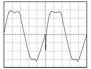
Shape. Repetitive waveforms should be symmetrical. That is, if you were to print the traces and cut them in two like-sized pieces, the two sides should be identical. A point of difference could indicate a problem.
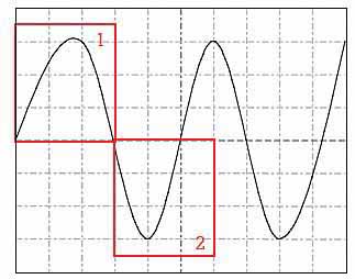 | Figure 8. If the two components of the waveform are not symmetrical, there may be a problem with the signal. |
Rising and falling edges. Particularly with square waves and pulses, the rising or falling edges of the waveform can greatly affect the timing in digital circuits. It may be necessary to decrease the time per division to see the edge with greater resolution.
 | Figure 9. Use cursors and the graticule marks to evaluate the rise and fall times of the leading and trailing edges of a waveform. |
Amplitude. Verify that the level is within the operating specifications of the circuit. Also check for consistency, from one period to the next. Monitor the waveform for an extended period of time, watching for any changes in amplitude.
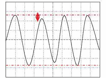 | Figure 10. Use horizontal cursors to identify amplitude fluctuations. |
Amplitude offsets. DC-couple the input and determine where the ground reference marker is. Evaluate any DC offset and observe if this offset remains stable or fluctuates.
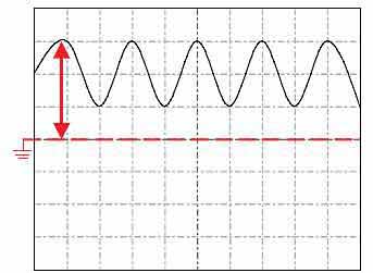 | Figure 11. Evaluate waveform DC offsets. |
Periodic waveshape. Oscillators and other circuits will produce waveforms with constant repeating periods. Evaluate each period in time using cursors to spot inconsistencies.
 | Figure 12. Evaluate period-to-period time changes. |
Waveform anomalies Here are typical anomalies that may appear on a waveform, along with the typical sources of such anomalies.
Transients or glitches. When waveforms are derived from active devices such as transistors or switches, transients or other anomalies can result from timing errors, propagation delays, bad contacts or other phenomena.
 | Figure 13. A transient is occurring on the rising edge of a pulse. |
Noise. Noise can be caused by faulty power supply circuits, circuit overdrive, crosstalk, or interference from adjacent cables. Or, noise can be induced externally from sources such as DC-DC converters, lighting systems and high-energy electrical circuits.
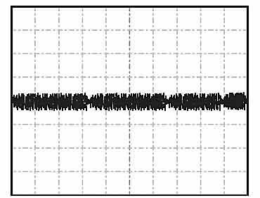 | Figure 14. A ground reference-point measurement showing induced random noise. |
Ringing.
Ringing can be seen mostly in digital circuits and in radar and pulse-width-modulation applications. Ringing shows up at the transition from a rising or falling edge to a flat DC level. Check for excessive ringing, adjusting the time base to give a clear depiction of the transitioning wave or pulse.
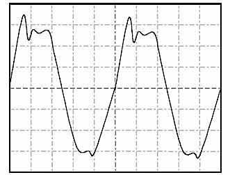 | Figure 15. Excessive ringing occurring on the top of the square wave. |
Momentary fluctuation. Momentary changes in the measured signal generally result from an external influence such as a sag or surge in the mains voltage, activation of a high-power device that is connected to the same electrical grid, or a loose connection. Use the DSO’s slowest timebase setting or the paperless recording or “roll” mode. Start at the input and watch the acquired waveform over long time spans to track down the source of the problem.
 | Figure 16a. A momentary change of approximately
1.5 cycles in the amplitude of the sinewave.
|
 | Figure 16b. Using an oscilloscope with a paperless recorder mode allows plotting of the amplitude (voltage level) over time. |
Drift. Drift — or minute changes in a signal’s voltage over time — can be tedious to diagnose. Often the change is so slow that it is difficult to detect. Temperature changes and aging can affect passive electronic components such as resistors, capacitors and crystal oscillators. One problematical fault to diagnose is drift in a reference DC voltage supply or oscillator circuit. Often the only solution is to monitor the measured value (V dc, Hz, etc.) over an extended time.
 | Figure 17. Performing a frequency measurement on a crystal oscillator that has been trend-plotted over an extended period (days or even weeks) can highlight the affect of drift caused by temperature changes and aging. |
Diagnosing problems Although successful troubleshooting is both an art and a science, adopting a troubleshooting methodology and relying on the functionality of an advanced DSO can greatly simplify the process.
Good troubleshooting practices will save time and frustration. The time-tested approach known as KGU, Known Good Unit comparison, accomplishes both goals. KGU builds on a simple principle: an electronic system that is working properly exhibits predictable waveforms at critical nodes within its circuitry, and these waveforms can be captured and stored. This reference library can be stored right on the DSO as an online resource, or can be printed out to serve as a hardcopy reference document. If the system or an identical system later exhibits a fault or failure, waveforms can be captured from the faulty system — called the device under test (DUT) — and compared with their counterparts in the KGU. Consequently, the DUT can either be repaired or replaced.
To build a reference library, start by identifying appropriate test points, or nodes, on the DUT. Now, run the KGU through its paces, capturing the waveform from each node. Annotate each waveform as required.
Get into the habit of always documenting key waveforms and measurements. Having a reference to compare to will prove invaluable during future troubleshooting
Troubleshooting
Whichever troubleshooting scenario below is appropriate at the time, remember that it’s important to inspect waveforms for fast-moving transients or glitches, even if a spot check of the waveform reveals no anomalies. These events can be difficult to spot, but the high sampling rate of today’s DSOs, together with effective triggering, makes it possible.
DUT with KGU. This approach assumes that you have access to a KGU and a reference library.
1. Make sure the DUT and KGU are set up in identical operating modes.
2. Starting at a high-level point in the system or block diagram, use the DSO to look for the presence or absence of fundamental signals. For example, look for a line-voltage supply, as well as subsequent DC supply voltages to the various subsystems. This requires probing the major input and output signals at major nodes in the system.
3. Compare signals at key nodes while changing the operating mode to see if a failure occurs. With signals from both devices available, you have two options:
• Display the live waveform from the KGU on Channel 1 of the DSO, and display the live waveform from the DUT on Channel 2.
• Capture a trace from the KGU and overlay it with a trace from the DUT. Perform a waveform-compare or pass/fail test.
4. Continue with this process until you note a variance between the DUT and KGU waveforms.
DUT with Circuit Diagrams. This approach assumes that no KGU and no waveform reference library for the DUT are available, but that circuit diagrams of the DUT can be located.
1. Review the circuit diagrams to understand the basic operation of the DUT.
• Analog circuits such as oscillators, amplifiers and signal conditioners (attenuators, filters and dividers) should exhibit uniform waveform patterns.
• Digital circuits such as gates, switches and processors should display waveforms with predictable amplitudes, pulse periods and even pulse patterns.
2. Starting at a high-level point in the system or block diagram, use the DSO to look for the presence or absence of fundamental signals. For example, look for a line-voltage supply, as well as subsequent DC supply voltages to the various subsystems. This requires probing the major input and output signals at major nodes in the system.
3. Use the storage capability of the DSO to capture and compare waveforms while changing the operating mode of the DUT.
• Visualize a theoretical “good” waveform and compare it to the waveform displayed on the DSO. Try to identify any obvious anomalies.
4. Use the horizontal or vertical cursors to quickly evaluate if the time or amplitude of the trace falls within the time or amplitude ranges suggested by the circuit design.
Complex DUT, No Circuit Diagrams. This approach assumes that the DUT is a fairly complex system, that no KGU is available, and that only limited DUT documentation is available.
1. Study the circuit cards, looking for common components and circuits, and identify highlevel test points in the system and check for the presence or absence of fundamental signals. As before, start at one point and work your way backwards probing the major input and output signals at major nodes in the system.
2. Compare waveforms at key nodes while changing the operating modes to see if a failure occurs. Store these waveforms.
3. If an examination of the DUT and analysis of waveforms at key circuit nodes reveal no obvious faults, use the DSO’s storage capability to solicit the aid of peers.
• Identify “suspect” waveforms from the DUT.
• Use the DSO’s Extract or Output mode to save these waveform files in a bitmap (.bmp) format.
• Email the files to a peer or factory expert anywhere in the world for aid in troubleshooting the circuit.
4. Using outside experts, go through each key node and one by one eliminate the obvious good nodes, eventually narrowing your focus to obvious faulty or suspect nodes.


